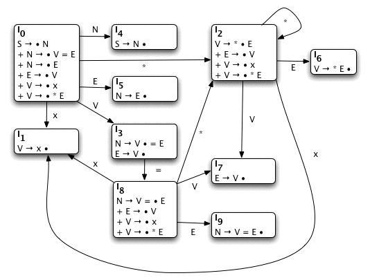
A pictoral representation of the Item Sets.
You may want to print this for quick reference.
Take two of a half-serious rant taken too far, by Stephen Jackson.
I've read several resources on syntax analysis. They left me with the impression that the topic was complex, and meant for minds greater than mine. But that didn't seem right. Learning how to use regular expressions to parse text is simple, and Context-Free Grammars in general aren't that much more complicated.
I believe that there is an easier way of explaining LALR(1) syntax analysis. This guide is my attempt to prove it.
I've decided that a "flashcard" method of explanation is for the best. Each "card" demonstrates a point or two, in a method that visually indicates all the text you should have to read to understand the point. If you get to the end of a card and you don't understand the point, just re-read the current card. Don't move on until you understand each card!
Enough background, let's get down to business.
For starters, you need to turn a string/file into a series of tokens during a phase referred to as "Lexical Analysis" which is outside the scope of this tutorial. The typical method of tokenizing is with regular expressions. A quick example of this would be the number 25 which would match the regular expression [0-9]+. We could then state that if input matches that expression, it should be classified as a num token.
Once we have a collection of tokens, we match them against a "grammar." Grammars are simple languages that are used to bootstrap more complex languages. They consist of simple mapping rules that indicate what rule to evaluate next (including self-references).
For example, rule binop could indicate a binary operation between two nums, such as +,-,*,/, etc. The notation commonly used for this is:
binop → num + num
      | num - num
      | num * num
      | num / num
From our earlier example, 25+25 would match the first rule of binop.
Any programmer worth their salt is probably annoyed with the repetition in the previous example. So let's create another mapping rule, operation to shorten the example:
binop → num operation num

operation → + | - | * | /
We now have a simple grammar to express a binary operation between two numbers. But why limit ourselves to only two numbers? In math, it is common to have many operators and numbers. In the meta-language of grammars, we add this quality with recursive rules:
binop → recbin operation num

recbin → recbin operation num
       | num

operation → + | - | * | /
Now we can express more complex equations such as 4/2-1*3+5.
We have to be careful defining recursive rules. To demonstrate this we'll make a temporary grammar that only maps a single num:
recdemo → num
But the grammar becomes invalid if we create a pointless, but logically resolvable rule:
recdemo → num
        | recdemo
Logically, the grammar's acceptable language is still {num}. We know that if you keep choosing recdemo you will just spin in an infinite loop until you choose num. Unfortunately, as logical as our computer is, it is incapable of resolving these two "equal" choices.
Another problem is when the correct path is not clear. The classic example of this is called the "Dangling Else" problem. Suppose we have two types of if statements. If statements, and if/else statements (like C).
code → if boolean code
     | if boolean code else code
     | arbitrarycode

boolean → true | false
Notice what happens when we follow an if's code, then find another if followed by an else? Which if does the else match?
The two possible matches are:
					if true if false arbitrarycode
					else arbitrarycode
if true if false arbitrarycode else arbitrarycode
We don't know which one is correct because the grammar is ambiguous.
Up until now, we've been implicitly treating binop as the starting state. But in a real grammar, we will need to explicitly declare a rule as the starting state. There is an additional requirement that a starting state must only have one token. To solve this, we'll make a start rule:
start → binop

binop → recbin operation num

recbin → recbin operation num
       | num

operation → + | - | * | /
A feature that won't be used in this tutorial is that a rule can have an empty option represented by the character "ε". Let's change the above example to accept a null string as input.
start → binop

binop → recbin operation num
      | ε

recbin → recbin operation num
       | num

operation → + | - | * | /
There is an alternative method to represent the above grammar:
start → binop

binop → recbin operation num
binop → ε

recbin → recbin operation num
recbin → num

operation → +
operation → -
operation → *
operation → /
While it is more verbose, it allows us to number each rule. We'll be using numbering to refer to specific rules (rather than constantly re-writing them).
Now that you are familiar with the concepts, there are some terms that you should know:
If you want to check your grammar there is a grammar checking tool online.
Now that you (hopefully) understand grammars, we can move onto processing them. The output of this phase (a parser) is a state machine to be used with source code.
The example grammar is simple, and a little redundant. Mainly for the sake of demonstration. The grammar is:
You may want to copy this grammar down (with the proper numbers) for later reference.
Item sets are collections of rules that have pointers to the current position of the rule. These pointers are usually denoted with a bullet (•). For example:
S → • N
S → N •
These cases indicate that N is about to be encountered, and that N has just been encountered, respectively.
The first item set, I0 begins with the starting rule,
S → • N
This means that we expect an N next. As a result,
we add all rules that map N, and because
N is next, we place the pointer at the start of the
N-rules.
S → • N
 + N → • V = E
 + N → • E
Both of the newly added items point to an unadded rule at their start, so we'll need to add the corresponding rules (V and E). Giving us I0:
S → • N
 + N → • V = E
 + N → • E
 + E → • V
 + V → • x
 + V → • * E
And because the pointers are only before terminals and non-terminals that we have already added, we have completed our first set.
To make the rest of the item sets, all we have to do is take the current item sets (only I0 at the moment) and then increment the pointer by giving it a specific input.
For example, what items in I0 expect an "x" next? Only
one, "V → • x". Thus, if we give
I0 an input of token "x" we will form a new item set
(I1) with only one item in it, the pointer will be
incremented past the given token.
I1:
V → x •
There is another rule in I0 that expects a terminal next
V → • * E. If we give I0 an input
of "*" we will begin a new set, I2:
V → * • E
Notice that the pointer is before the non-terminal E. Thus we need to add all E-rules.
V → * • E
 + E → • V
Again, there is a pointer before the non-terminal V. Like E earlier, we need to add all V-rules. This gives us the final item set.
I2:
V → * • E
 + E → • V
 + V → • x
 + V → • * E
There are two things to notice about this set. The first is that if we give this set an input of "x" we return to I1 (Sets are not duplicated).
The second thing to notice is that because of the last rule, if you give this set an input of "*" we return to this set.
The next step is giving I0 an input of V. It forms an item set with multiple rules.
I3:
N → V • = E
E → V •
Try doing the next few sets on your own. If you get stuck, the answers will be given on this card. Remember that once you finish giving input to the current item set (I0) you need to move onto the next item set that requires input (I2), and so on until you have created a set dealing with every possible input.
I4:
S → N •
I5:
N → E •
I6:
V → * E •
I7:
E → V •
I8:
N → V = • E
 + E → • V
 + V → • x
 + V → • * E
I9:
N → V = E •
A pictoral representation of the Item Sets.
You may want to print this for quick reference.
To construct the Translation Table all we need to do is determine what item set to go to next based on a given input.
For example, I0:
S → • N
 + N → • V = E
 + N → • E
 + E → • V
 + V → • x
 + V → • * E
As stated before, if we give I0 an input of x we end up in item set 1 (I1). Thus, we have our first piece of the transition table:
| Item Set | x |
|---|---|
| 0 | 1 |
If we give I0 a '=' then nothing occurs. But a '*' leads to I2. Which gives us a larger piece of the transition table:
| Item Set | x | = | * |
|---|---|---|---|
| 0 | 1 | 2 |
We just need to repeat this process over all item sets and inputs.
Here is the resulting transition table for our grammar:
| Item Set | x | = | * | S | N | E | V |
|---|---|---|---|---|---|---|---|
| 0 | 1 | 2 | 4 | 5 | 3 | ||
| 1 | |||||||
| 2 | 1 | 2 | 6 | 7 | |||
| 3 | 8 | ||||||
| 4 | |||||||
| 5 | |||||||
| 6 | |||||||
| 7 | |||||||
| 8 | 1 | 2 | 9 | 7 | |||
| 9 |
For the next phase we are going to have to traverse the item sets previously created. To explain this quickly we'll have to introduce a shorthand notation.
For example, if we wanted to start in I0 and follow the
rule V → * E.
We would start by giving I0 a *. According to the picture above, this would lead to I2. We express this as 0*2
The next step, I2 to I6 due to E. Where the shorthand form is 2E6
To get the last component of the rule we need to determine the left-hand side. The non-terminal is V and if we give I0 an input of V we go to I3. Denoted as 0V3
Putting them altogether gives us a "new" rule: 0V3 → 0*2 2E6
Fortunately, we only need to do this with rules that start with a pointer. Giving us our extended grammar:
Steps to Make the First Set
V → x where the first symbol is
a terminal, First(V) contains x. In a similar case,
V → ε, First(V) would contain ε.
R → A B C), then we would start by adding
First(A) (minus ε) to First(R). If First(A) contained
ε we would add First(B) to First(R), and so on.Step 1 isn't really used (I only explained it to avoid an ambiguity within step 3). All we have to do is apply step 2 to all rules, then step 3.
Let's make the First Set for our grammars.
Starting with step 2, it only applies to rules 4 and 5 of our original grammar, and therefore only impacts rules 1, 2, 7, 8, 9, and 10 in the extended grammar.
Original Grammar: First(V) = { x, * }
Extended Grammar:
					First(0V3) =
					{ x, * }

					First(2V7) =
					{ x, * }

					First(8V7) =
					{ x, * }
Because the first symbol of V is always a terminal, we have finished determining all the variations of First(V).
Step 3 will be the one to determine the remainder of the sets. Since we have First(V) of our original grammar and by step 3 we know that First(E) is going to be the same as First(V).
First(E) = First(V) = { x, * }
In our extended grammar, the same principle is used, but over more rules.
					First(0E5) =
					First(0V3) =
					{ x, * }


					First(2E6) =
					First(2V7) =
					{ x, * }


					First(8E9) =
					First(8V7) =
					{ x, * }
From the "general rule" (our original grammar) we have First(E) and First(V) we can determine First(N).
First(N) = First(E) union First(V) = { x, * }
our earlier mappings show it is the same as:
First(N) = First(E) = First(V) = { x, * }
Finally, we can compute First(S):
First(S) = First(N) = { x, * }
Likewise, the extended grammar only has one S and
N rule:
					First(0S$) =
					First(0N4) =
					First(0E5) =
					First(0V3) =
					{ x, * }
The first set of every non-terminal in both grammars is:
{ x, * }
Steps to Make the Follow Set
Conventions: a, b, and c represent a terminal or non-terminal. a* represents zero or more terminals or non-terminals (possibly both). a+ represents one or more... D is a non-terminal.
R → a*Db. Everything in
First(b) (except for ε) is added to Follow(D). If First(b)
contains ε then everything in Follow(R) is put in Follow(D).
R → a*D,
then everything in Follow(R) is placed in Follow(D).
Let's apply the steps, starting with 1, putting $ in S's follow set.
Follow(S) = { $ }
Step 2 on rule 1 (N → V = E) indicates that
first(=) is in Follow(V).
Because of step 3 on rule 5 (V → * E):
Follow(E) = Follow(V)
Interestingly enough, step 3 on rule 4 (E → V)
creates a symmetrical relationship:
Follow(V) = Follow(E)
And step 3 on rules 0 and 2 (S → N and
N → E) spread Follow(S) to the follow sets of the
other non-terminals. Giving us a final result:
					Follow(S) = { $ }

					Follow(N) = { $ }

					Follow(E) = { $, = }

					Follow(V) = { $, = }
Now that you know how to do it on the original grammar, try it on the extended grammar. Here are the results:
					Follow(0S$) =
					{ $ }

					Follow(0N4) =
					{ $ }

					Follow(0E5) =
					{ $ }

					Follow(8E9) =
					{ $ }

					Follow(2E6) =
					{ $, = }


					Follow(0V3) =
					{ $, = }


					Follow(8V7) =
					{ $ }

					Follow(2V7) =
					{ $, = }
We create the action/goto table by using the output of previous goals. There are only four steps for this goal:
Step 1 - Initialize
Add a column for the end of input, labelled $.
Place an "accept" in the $ column whenever the item set contains an
item where the pointer is at the end of the starting rule (in
our example "S → N •").
Step 2 - Gotos
Directly copy the Translation Table's nonterminal columns as GOTOs.
Step 3 - Shifts
Copy the terminal columns as shift actions to the number determined from the Translation Table. (Basically we just copy the transition table, but we put an "s" in front of each number, see below.)
Step 4 - Reductions, Sub-Step 1
Earlier on we determined the Follow Sets of the extended grammar. Now we need to combine the two. We start this process by matching the follow sets to an extended rule's left-hand side.
| Number | Rule | Follow Set |
|---|---|---|
| 0 | 0S$ → 0N4 | { $ } |
| 1 | 0V3 → 0x1 | { $, = } |
| 2 | 0V3 → 0*2 2E6 | { $, = } |
| 3 | 0N4 → 0E5 | { $ } |
| 4 | 0N4 → 0V3 3=8 8E9 | { $ } |
| 5 | 0E5 → 0V3 | { $ } |
| 6 | 2E6 → 2V7 | { $, = } |
| 7 | 2V7 → 2x1 | { $, = } |
| 8 | 2V7 → 2*2 2E6 | { $, = } |
| 9 | 8V7 → 8x1 | { $ } |
| 10 | 8V7 → 8*2 2E6 | { $ } |
| 11 | 8E9 → 8V7 | { $ } |
We can merge rules that decend from the same original rule, and have
the same end point (the very last transition number). From the
above grammar, we can merge rules 6 and 11 into a common rule (we
no longer need to keep all the transition numbers, just the final
number, which is 7 due to
...V7 in this
case).
They will have the union of the follow sets.
Leading to the row:
| Final Set | Pre-Merge Rules |
Rule | Follow Set |
|---|---|---|---|
| 7 | 6, 11 | E → V | { $, = } |
Notice that number 5, 0E5 → 0V3, is left out even though it decends from the same rule as 6 and 11? That is because they have a different endpoint (final set).
Step 4 - Reductions, Sub-Step 2
Here are tuples consisting of the merged rules, their origin, follow sets, and final set:
| Final Set | Pre-Merge Rules |
Rule | Follow Set |
|---|---|---|---|
| 1 | 1, 7, 9 | V → x | { $, = } |
| 3 | 5 | E → V | { $ } |
| 4 | 0 | S → N | { $ } |
| 5 | 3 | N → E | { $ } |
| 6 | 2, 8, 10 | V → * E | { $, = } |
| 7 | 6, 11 | E → V | { $, = } |
| 9 | 4 | N → V = E | { $ } |
Final Set 4, S → N is a special case where the
reduction leaves us with nothing, and is thus considered accepting.
Since this case is handled in step 1, we ignore this rule during the
reduction phase.
We can then rearrange the remaining tuples to form a reduction table. The columns are the contents of the used follow sets { $, = } and the final set numbers.
| Final Set | $ | = |
|---|---|---|
| 0 | ||
| 1 | V → X |
V → X |
| 2 | ||
| 3 | E → V |
|
| 4 | ||
| 5 | N → E |
|
| 6 | V → * E |
V → * E |
| 7 | E → V |
E → V |
| 8 | ||
| 9 | N → V = E |
Merge Steps: Result
The previous steps give us the Action/Goto table:
| Action | Goto | |||||||
|---|---|---|---|---|---|---|---|---|
| Item Set | $ | x | = | * | S | N | E | V |
| 0 | s1 | s2 | 4 | 5 | 3 | |||
| 1 | r(V → x) |
r(V → x) |
||||||
| 2 | s1 | s2 | 6 | 7 | ||||
| 3 | r(E → V) |
s8 | ||||||
| 4 | accept | |||||||
| 5 | r(N → E) |
|||||||
| 6 | r(V → * E) |
r(V → * E) |
||||||
| 7 | r(E → V) |
r(E → V) |
||||||
| 8 | s1 | s2 | 9 | 7 | ||||
| 9 | r(N → V = E) |
|||||||
In this table you'll see the term "Item Set" used. But after this point the term "state" will become more appropriate. The two terms will be used interchangeably.
An alternative representation of the previous table, the one we will use to parse input, will be constructed by replacing the reduction rules with the original rules' numbers, rather than the rules.
| Action | Goto | |||||||
|---|---|---|---|---|---|---|---|---|
| State | $ | x | = | * | S | N | E | V |
| 0 | s1 | s2 | 4 | 5 | 3 | |||
| 1 | r4 | r4 | ||||||
| 2 | s1 | s2 | 6 | 7 | ||||
| 3 | r3 | s8 | ||||||
| 4 | accept | |||||||
| 5 | r2 | |||||||
| 6 | r5 | r5 | ||||||
| 7 | r3 | r3 | ||||||
| 8 | s1 | s2 | 9 | 7 | ||||
| 9 | r1 | |||||||
At this point, I'd like to mention some terminology. This algorithm generates an LALR-by-SLR, LR parse table. The only things that are uniquely "LALR(1)" are the reductions and the result. The algorithm used to parse it in the next section is just an LR parser.
Another thing I'd like to mention is that I think this guide teaches the subject bottom-up instead of top-down. But you may need to read a formal guide before you see the (slight) pun in this comment.
Using the grammar and Action/Goto table from the previous section, we will parse the string x = * x.
There are three elements we need to keep track of while parsing the stack:
A fourth element that we don't need to keep track of, but will be of assistance in the explanation of the parser is "Next Action."
In each state there are four possible options:
|
Now that we know the rules, let's walk through the first steps in our example x = * x. The first step is to initialize the table:
The first token we encounter in state 0 is an x, which indicates that a shift to state 1 is in order. The first x is removed from the input, and 1 is placed on the stack. Leading us to the next row in the table:
Reducing by rule 4 will put a 4 in the output. Rule 4,
Now that the two main operations (shift and reduce) have been demonstrated, you can try to do the rest of the table yourself. If you get into trouble, the result is below:
|
A Handy ReferenceRules
Parse Table
|
||||||||||||||||||||||||||||||||||||||||||||||||||||||||||||||||||||||||||||||||||||||||||||||||||||||||||||||||||||||||||||||||||||||||||||||||||||||||||||||||||||||||||||||||||||||||||||||||
In our example of x = * x we get the output 4, 4, 3, 5, 3, 1. To review, we'll construct objects based on the example.
When the first reduction occurred (r4) we had just inputted the
terminal x. By rule 4, V → x, x mapped
onto the non-terminal V. Thus we have our first object,
V(x).
The second time a reduction occurs (r4) is just after we've inputted the entire string meaning that we are turning the last x into a V. Which gives us our second object, V(x). At this point we can re-substitute our objects back into the string, which gives us V(x) = * V(x).
Reduction 3 just maps the last V(x) into E(V(x)). Giving us V(x) = * E(V(x)).
The remaining mappings are:
It is a cumbersome way of looking at it. But it shows how to map the LR parsing method into constructors. And if we give each rule a function, then it should be obvious how to generate code. For example, V(x) could be used to make token x into an object of type V. Any object of type E is formed by giving the constructor an object of type V. And so on until we reach the eventual end of this example by creating an object of type S by giving it an object of type N.
This document was written by Stephen Jackson, © 2009.
Feel free to copy, modify, distribute, or link this document. I just ask for fair credit if you use my work.
If you've gotten this far and are looking for something else to do, drop me a line (My email is here) with your opinion of this tutorial.